PyTransit Quickstart#

PyTransit comes with a set of transit models that share a common interface (API). However, except for some specific use-cases, you will pretty much always want to use the RoadRunner Model (or RRModel for short). The details of the model can be found from the RoadRunner-specific example notebooks, but these examples should help you to get started.

[1]:

%matplotlib inline

[22]:

from matplotlib import rc
from matplotlib.pyplot import setp, subplots
from numpy import linspace, pi, tile, repeat, arange
from numpy.random import uniform, normal, seed

[3]:

rc('figure', figsize=(13,5))

def plot_lc(time, flux, c=None, ylim=(0.9865, 1.0025), ax=None):
    if ax is None:
        fig, ax = subplots()
    else:
        fig, ax = None, ax
    ax.plot(time, flux, c=c)
    ax.autoscale(axis='x', tight=True)
    setp(ax, xlabel='Time [d]', ylabel='Flux', xlim=time[[0,-1]], ylim=ylim)

    if fig is not None:
        fig.tight_layout()
    return ax

Model import#

First, we need to import the RoadRunner Model from PyTransit.

[4]:

from pytransit import RRModel

Model initialisation#

After the import, the transit model needs to be initialised and set up. Here we first create a RoadRunnerModel uses the power-2 limb darkening law and set it up by giving it a set of mid-exposure times. Both the model initializer and the set_data method have plenty of additional optional arguments for more advanced model setups, but here we aim for simplicity.

[5]:

tm = RRModel('power-2')
tm.set_data(time = linspace(-0.05, 0.05, 500))

Basic evaluation#

After the transit model has been initialised, it can be evaluated using the evaluate method. The method arguments are

k: the planet-star radius ratio,
ldc: limb darkening model coefficients,
t0: the zero epoch,
p: the orbital period,
a: the orbital semi-major axis divided by the stellar radius,
i: the orbital inclination in radians,
e: the orbital eccentricity (optional, can be left out if assuming circular a orbit), and
w: the argument of periastron in radians (also optional, can be left out if assuming circular a orbit).

Note: The first model evaluation will take some time because Numba needs to compile the model. The evaluation will be very fast after the first evaluate call.

Note: The model initialization takes

[6]:

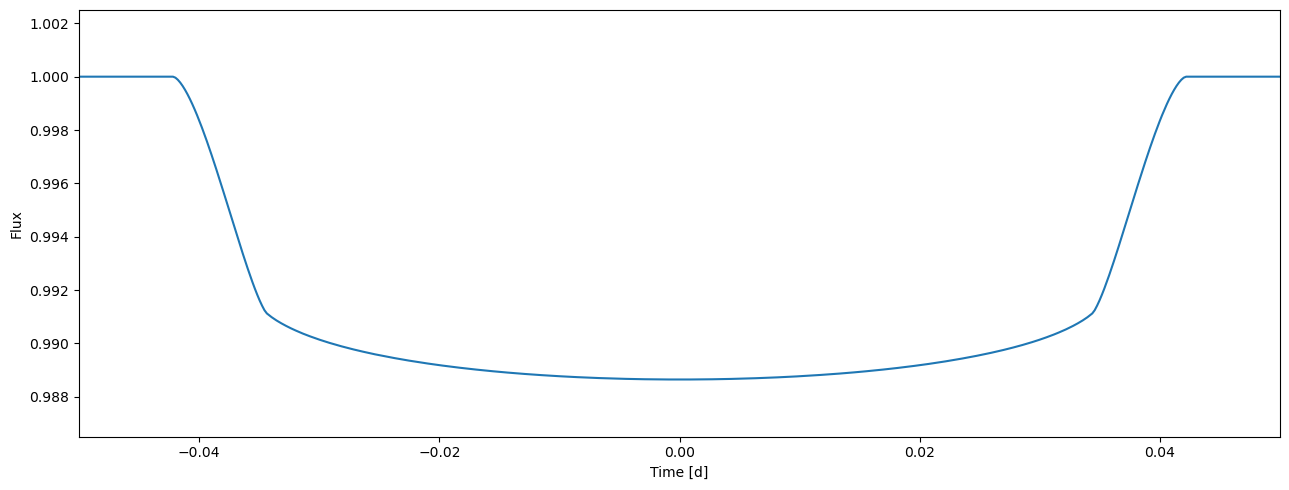
flux = tm.evaluate(k=0.1, ldc=[0.6, 0.5], t0=0.0, p=1.0, a=4.2, i=0.5*pi, e=0.0, w=0.0)
plot_lc(tm.time, flux);

Evaluation for a set of parameters#

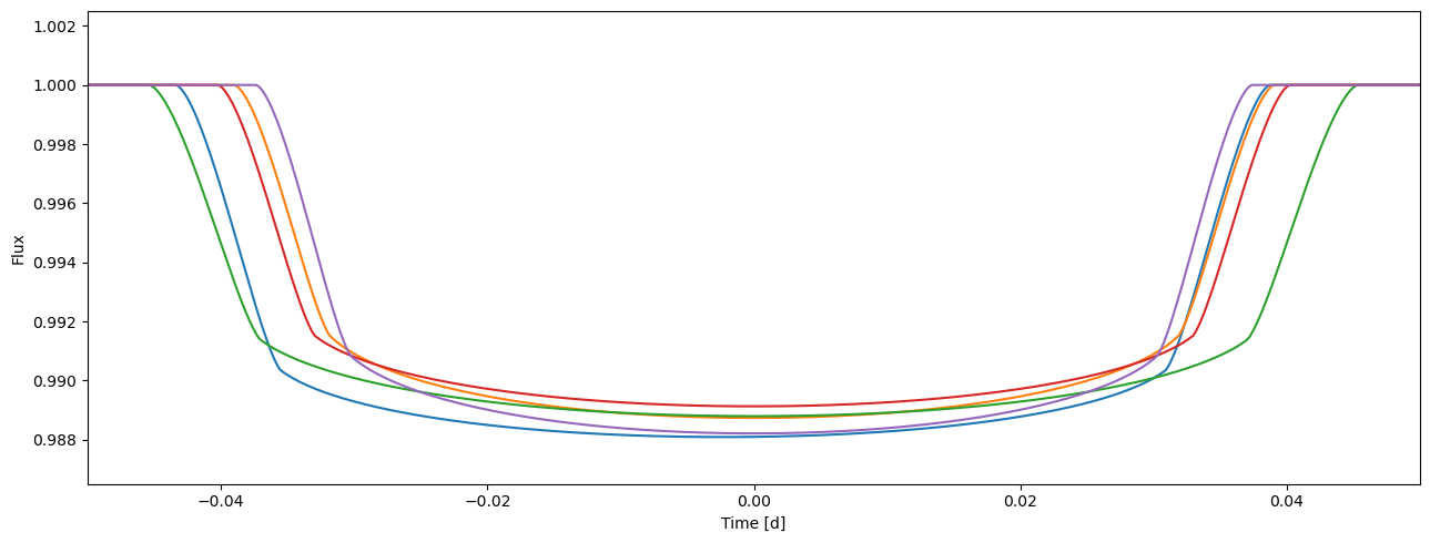
In the most simple case the limb darkening coefficients are given as a single vector and the rest of the parameters are scalars, in which case the flux array will also be one dimensional. However, if we want to evaluate the model for multiple parameter values (such as when using emcee for MCMC sampling), giving a 2D array of limb darkening coefficients and the rest of the parameters as vectors allows PyTransit to evaluate the models in parallel, which can lead to significant performance improvements (especially with the OpenCL versions of the transit models). Evaluating the model for n sets of parameters will result in a flux array with a shape (n, time.size).

Note: The first model evaluation will again take some time because Numba needs to compile the model optimised for a parameter set. The evaluation will be very fast after the first evaluate call.

[7]:

npv = 5
seed(1)
ks    = normal(0.10, 0.002, (npv, 1))
t0s   = normal(0, 0.001, npv)
ps    = normal(1.0, 0.01, npv)
smas  = normal(4.2, 0.1, npv)
incs  = uniform(0.49*pi, 0.5*pi, npv)
es    = uniform(0, 0.15, size=npv)
ws    = uniform(0, 2*pi, size=npv)
ldc   = uniform(0.5, 0.7, size=(npv,1,2))

[10]:

flux = tm.evaluate(ks, ldc, t0s, ps, smas, incs, es, ws)
print(flux.shape)
plot_lc(tm.time, flux.T);

(5, 500)

../_images/notebooks_quickstart_12_1.png

Adding complexity: Heterogeneous data sets and variations in model parameters#

Basics#

Ok, modeling a simple transit light curve is easy, but what to do if we want to model a set of light curves observed in different passbands or with very different exposure times (such as when modeling long-cadence Kepler or TESS observations with short-cadence observations, or with ground-based photometry)? And what to do if the orbital parameters of the planet vary in time?

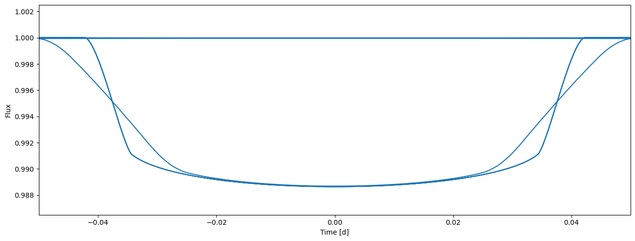
In PyTransit, each exposure is associated with a light curve index (lcid). Exposures with a common light curve index are considered to belong to a single homogeneous light curve.

Modeling different observing cadences#

[32]:

time = tile(linspace(-0.05, 0.05, 500), 3)
lcids = repeat(arange(3), 500)

[33]:

tm.set_data(time, lcids=lcids, nsamples=[1, 10, 1], exptimes=[0.0, 0.02, 0.0])

[34]:

flux = tm.evaluate(k=0.1, ldc=[0.6, 0.5], t0=0.0, p=1.0, a=4.2, i=0.5*pi, e=0.0, w=0.0)
plot_lc(tm.time, flux);

../_images/notebooks_quickstart_16_0.png

PyTransit Quickstart

Contents